Making an Upset plot

To visualize the results, we need to visualize associations between genera, and the number of times these links were found in the database. The matrix layout under the barplot allows UpsetR to effectively visualize these links.

To run UpsetR, we first need to process the data we collected previously, so that it is in a format that UpsetR can work with. Specifically, we will make a column filled with zeroes for each genus. Each association is encoded as a row. Values in the row are set to 1 depending on the genera participating in that association. We will also remove the other columns, since those cannot be used directly by UpsetR, but need to be added via a metadata dataframe. When running the code below, make sure to change the input and output parameters so they match the location of the exported data.

library(UpSetR)
library(viridis)

input <- "C:/Users/username/Input"
output <- "C:/Users/username/Output"

data <- read.csv(file.path(input, "propionate_matches.csv"), row.names="X", stringsAsFactors=FALSE)

upset_data <- data
for (target in data$Sugar.degradation){
  upset_data[[target]] <- 0
}
for (target in data$Propionate.formation){
  upset_data[[target]] <- 0
}
upset_data$Sugar.degradation <- NULL
upset_data$Propionate.formation <- NULL
upset_data$Network <- NULL

for (i in 1:nrow(data)){
  row <- data[i,]
  sugar_degrader <- data$Sugar.degradation[i]
  upset_data[[sugar_degrader]][i] <- 1
  propionate_producer <- data$Propionate.formation[i]
  upset_data[[propionate_producer]][i] <- 1
}

Next, we will create the metadata dataframe, so we can represent the molecules linked to each of the genera according to literature. We will also define some colorblind-friendly colours.

metadata <- data.frame(Sets=c("Lactobacillus",
                              "Bacteroides",
                              "Escherichia",
                              "Blautia",
                              "Anaerostipes",
                              "Roseburia",
                              "Clostridium",
                              "Listeria"))
metadata$Substrate <- c('lacp',
                        'fuc',
                        'fucother',
                        'fucp',
                        'fuc',
                        'fucp',
                        'other',
                        'fucp')
# need to manually define sets
colours <- viridis(5)

The last part is then to create the Upset plot and save it to a PDF file.

pdf(file=file.path(output, "Figure2b_propionate_matches.pdf"), width=6, height=5, onefile=FALSE) 
upset(upset_data, nsets=20, 
      set.metadata = list(data=metadata, 
      plots=list(list(type="matrix_rows", column="Substrate", alpha=0.5,
      colors=c(fuc = colours[[1]], 
      fucp = colours[[2]],
      lacp = colours[[3]],
      other = colours[[4]],
      fucother = colours[[5]])))))
dev.off()

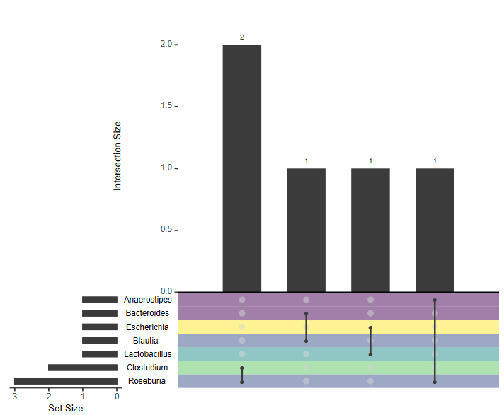
The results should look similar to the image below, although these values are only shown for 5 Animal data sets. Here, Roseburia had the most associations that could potentially be linked to propionate production. We later manually added a legend that visualized the propionate pathway.